Environmental science / Atmospheric science / Data analysis
Environmental data. Atmospheric insight.
I’m Aseem Sharma, an environmental science student at the University of Houston with an atmospheric science concentration and a mathematics minor. My work combines programming, spatial analysis, and numerical modeling to investigate air quality and weather.
01 / TCEQ · Air Modeling & Data Analysis · Summer 2026
Preparing emissions data for air-quality modeling
I converted legacy SAS workflows into R and Python to process MOVES5 and TEXN2 emissions-model data for EPS3 PREAM inputs. The work translated large model datasets into the format needed for downstream air-quality modeling.
R
Python
Bash
Matplotlib
Unix
49 statesMOVES5 coverage outside Texas
254 countiesTEXN2 coverage across Texas
My contribution and workflow
Implementation
I reimplemented the processing logic in R for MOVES5 and Python for TEXN2, working with millions of emissions-model records. I worked in AMDA’s Unix server environment and used Python and Matplotlib for supporting summaries and visualizations.
Deliverable
The workflows produced EPS3 PREAM outputs for downstream modeling. This experience strengthened my ability to interpret established scientific code, transform large datasets, and check outputs against modeling requirements.
02 / Geospatial Analysis and Applications · Houston air quality · Group project · Spring 2026
Mapping ozone and social vulnerability in Houston
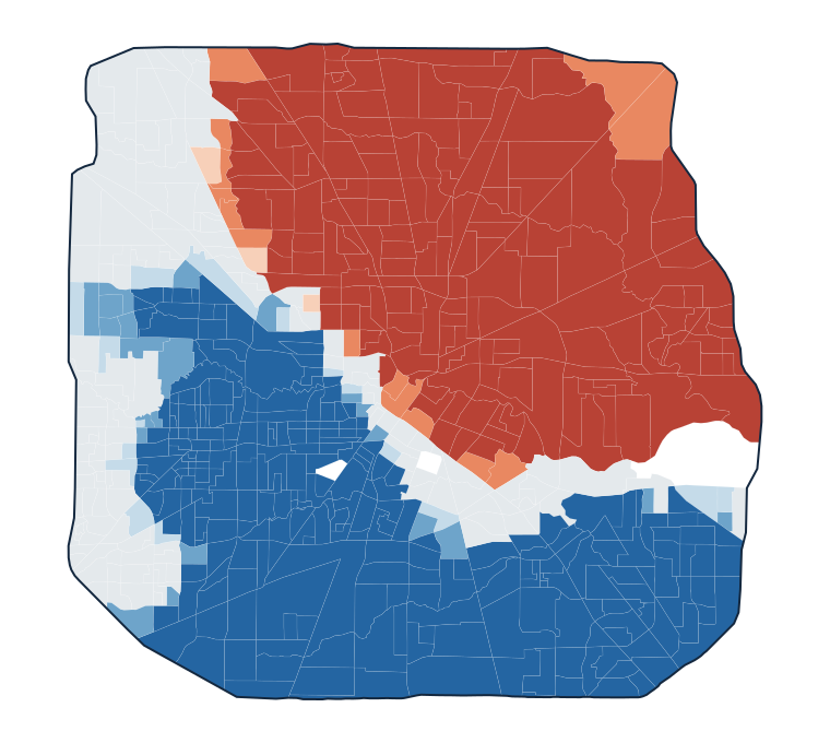
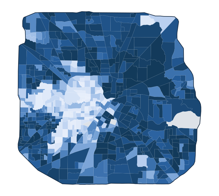
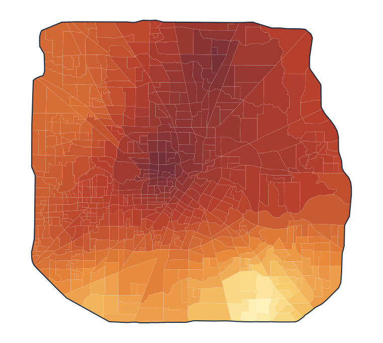
Our project examined how modeled ozone patterns overlap with social vulnerability and asthma prevalence within Houston’s Beltway 8. We combined EPA monitoring data with census-tract indicators to investigate the spatial distribution of environmental and social burdens.
ArcGIS Pro
Ordinary kriging
Zonal statistics
Getis-Ord Gi*
Spatial analysis
Key finding
The summer ozone–SVI analysis identifies a broad cluster of higher composite values in northeastern and eastern Houston, with lower-value clusters toward the west and south. This geographic pattern supports closer investigation of monitoring coverage and the conditions affecting vulnerable communities.
Summer ozone–SVI composite clusters. Red represents statistically significant high-value clusters and blue represents low-value clusters; gray indicates no significant clustering. Darker shades indicate higher confidence (90%, 95%, and 99%).Methods, supporting maps, and interpretation
Study scope
The broader project considered ozone alongside both social vulnerability and asthma prevalence. The maps displayed here focus on the summer ozone–SVI analysis.
Social vulnerability. Census-tract overall SVI percentile ranks, from 0 to 1; higher values indicate greater relative vulnerability. Gray indicates missing data.Estimated summer ozone. Census-tract means from the interpolated surface range from 38.55 to 43.41 ppb. Gray indicates missing data.
Workflow
Prepare: Assemble ozone monitoring summaries and census-tract social vulnerability data within the study area.
Interpolate: Estimate the summer ozone surface with ordinary kriging and summarize it by census tract using zonal statistics.
Combine: Standardize ozone and SVI as z-scores and average them with equal weight.
Analyze: Identify spatial clusters with Getis-Ord Gi* using a 9 km distance band, Euclidean distance, and row standardization.
Interpretation
These maps describe relative patterns in a combined index. A high composite value does not necessarily mean both components are individually high, and the clusters do not establish personal exposure, regulatory exceedances, or a causal health effect.
Sparse monitoring limits local detail, interpolation smooths variation, and census-tract aggregation can mask differences within neighborhoods. The cluster analysis does not apply a false-discovery-rate correction. Additional monitoring and temporal analysis would help assess the stability of these patterns.
Team: Aaron Ehlert, Logan Husbands, Heather Meyers, Fernando Sarmiento-Cala, and Aseem Sharma.
03 / Numerical Modeling in Atmospheric Sciences · Spring 2025
Simulating Hurricane Harvey with nested WRF domains
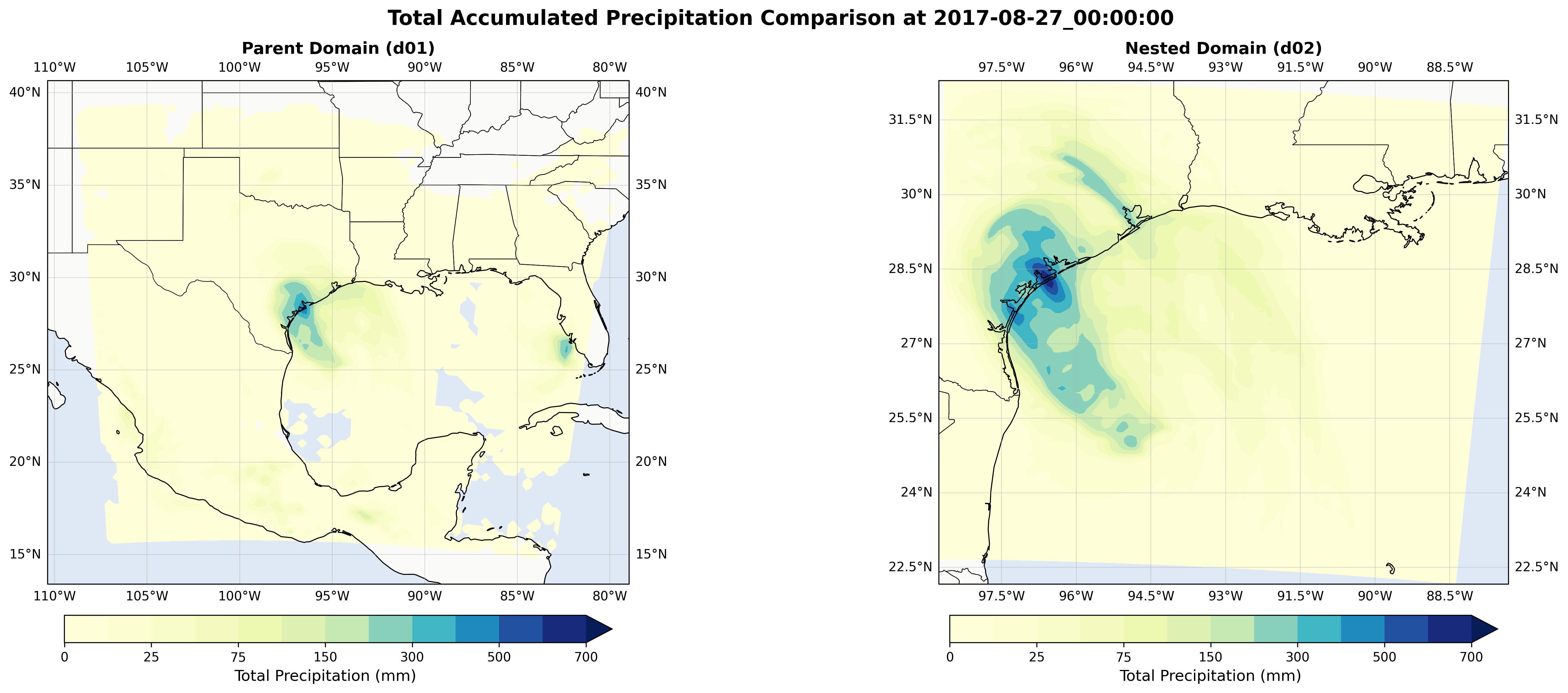
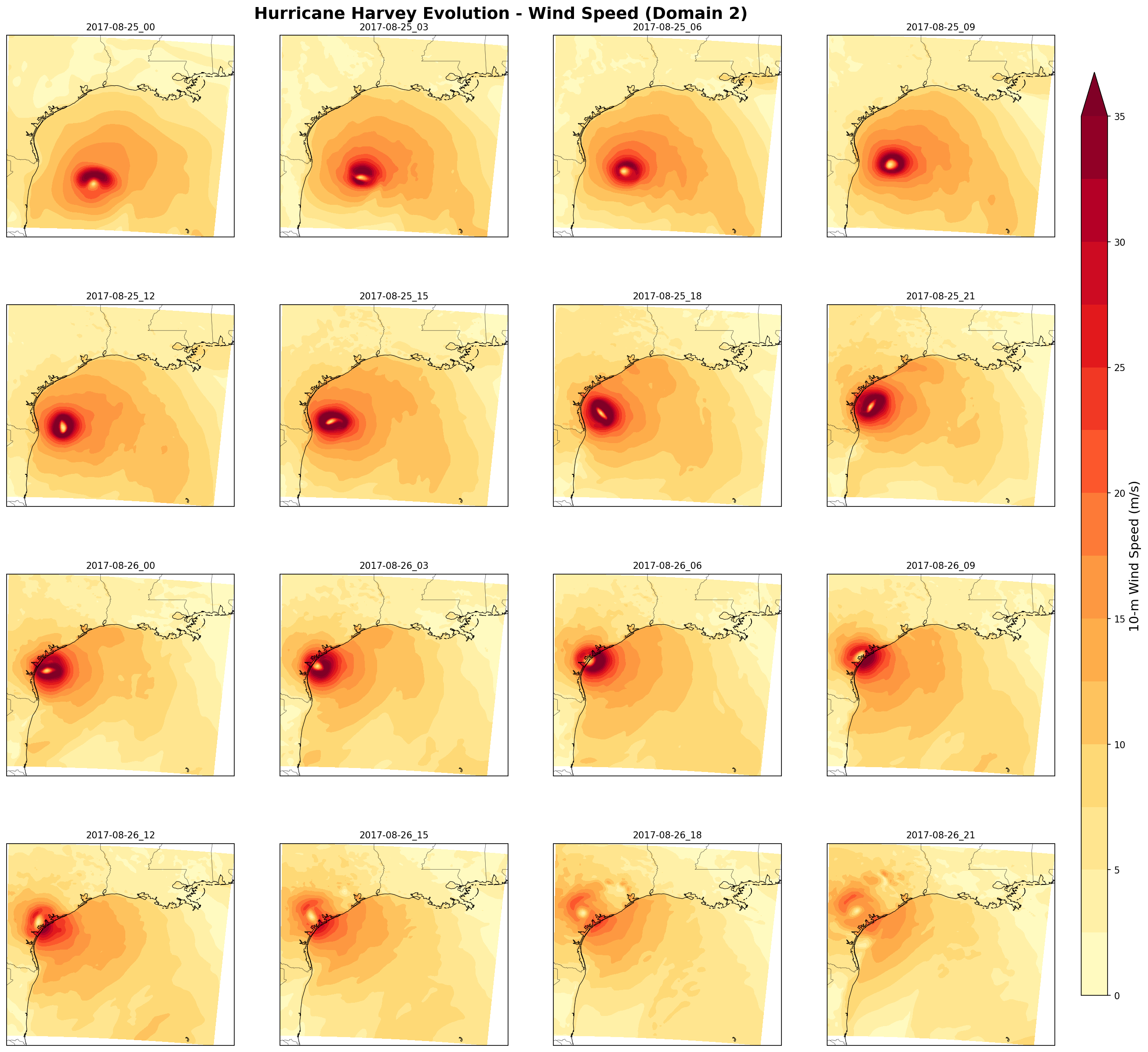
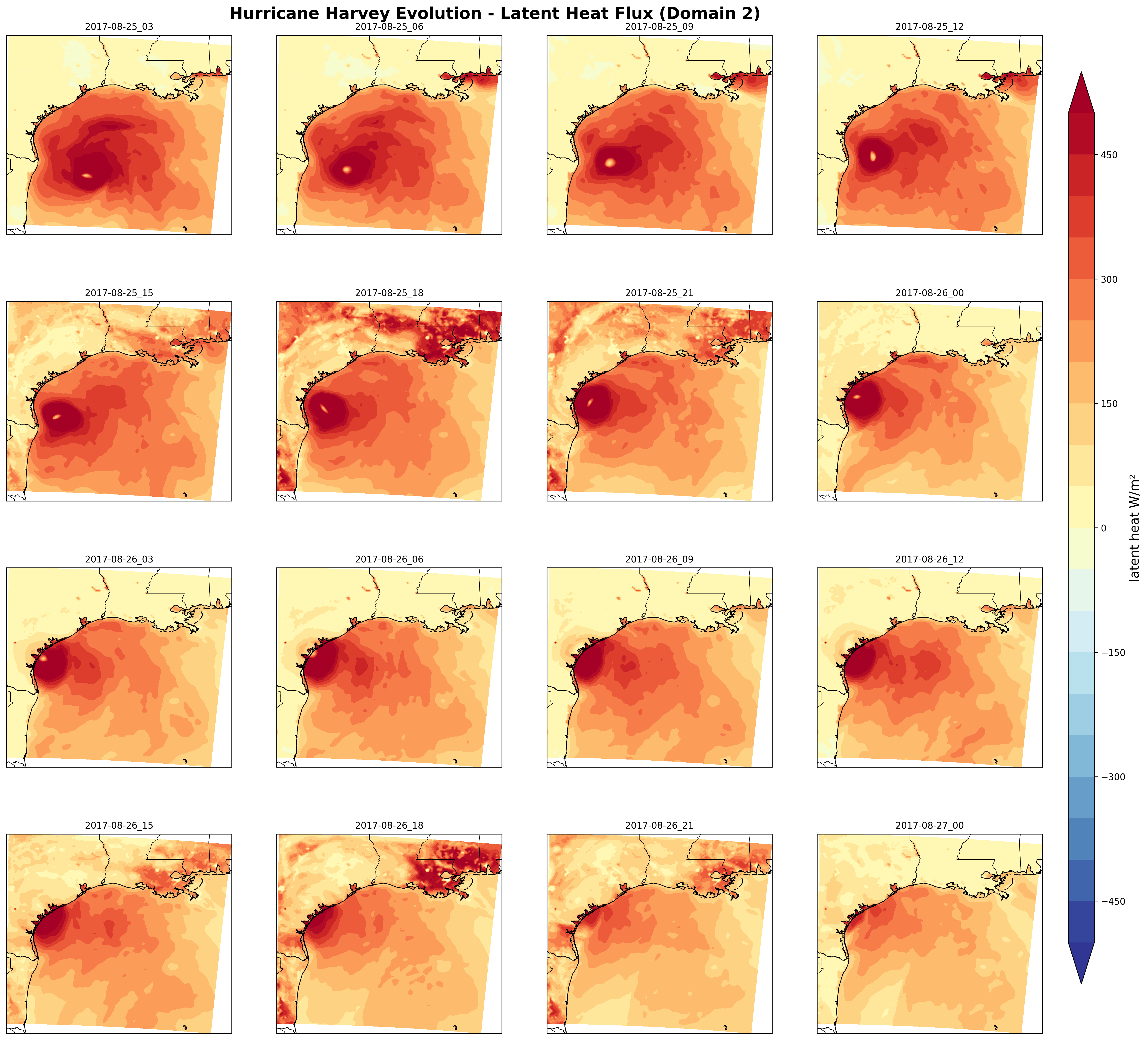
I completed a WRF modeling and visualization project for August 25–27, 2017, using a 27 km parent domain and a 9 km nested domain. I analyzed the output in a Jupyter notebook to compare accumulated precipitation and examine wind and surface-flux evolution.
WRF / WPS
Python
xarray
NumPy
Matplotlib
Cartopy
Jupyter
What the simulation showed
The analysis produced maximum accumulated precipitation of 452.0 mm in the parent domain and 671.6 mm in the nested domain at the final output time. The finer domain resolves a more localized precipitation maximum in the displayed simulation. These are modeled totals over different domain extents, not observed rainfall or a measure of forecast accuracy.
Accumulated RAINC + RAINNC at August 27, 2017, 00 UTC. The configured run starts August 25 at 00 UTC and uses no restart. This comparison covers the modeled interval, not Harvey’s full event rainfall.Explore the configuration, workflow, and evolution maps
My work
I completed the model setup, run, and output analysis for the course project. I used WRF and WPS namelists to configure the simulation, checked run completion, and analyzed the output in Python.
Configuration
The model configuration specifies two domains with a 3:1 nesting ratio, 45 vertical levels, hourly output, and a 48-hour integration. Feedback from the nest to the parent is disabled. The output inventory contains 49 hourly files per domain, including both endpoints.
Analysis
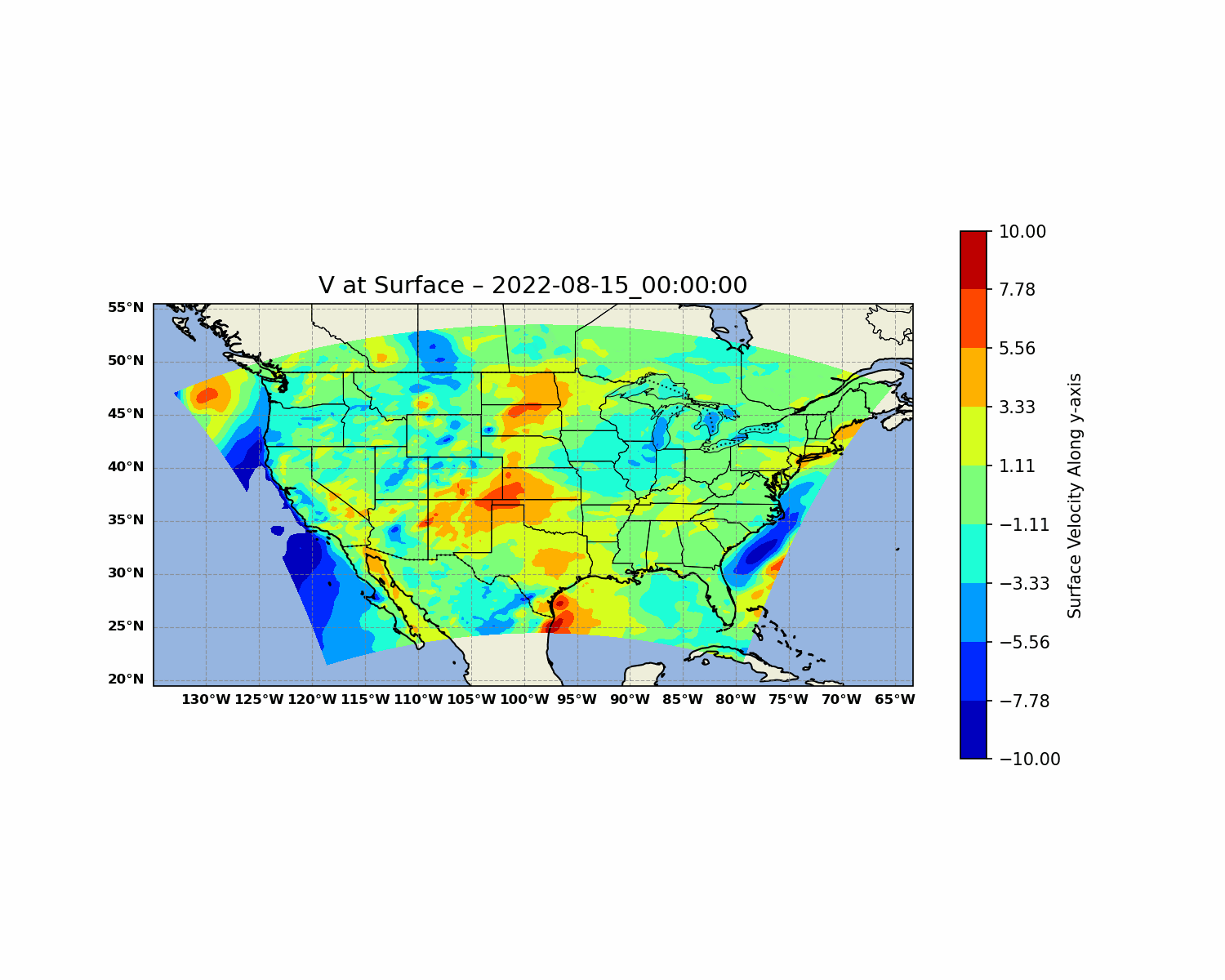
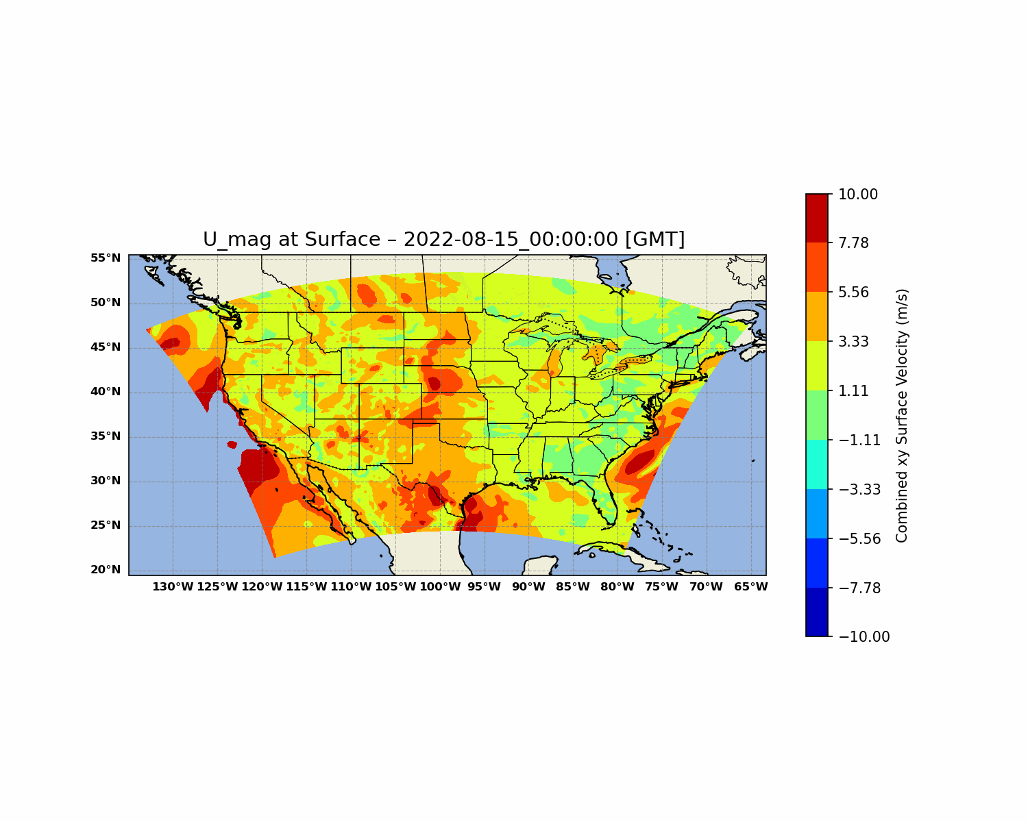
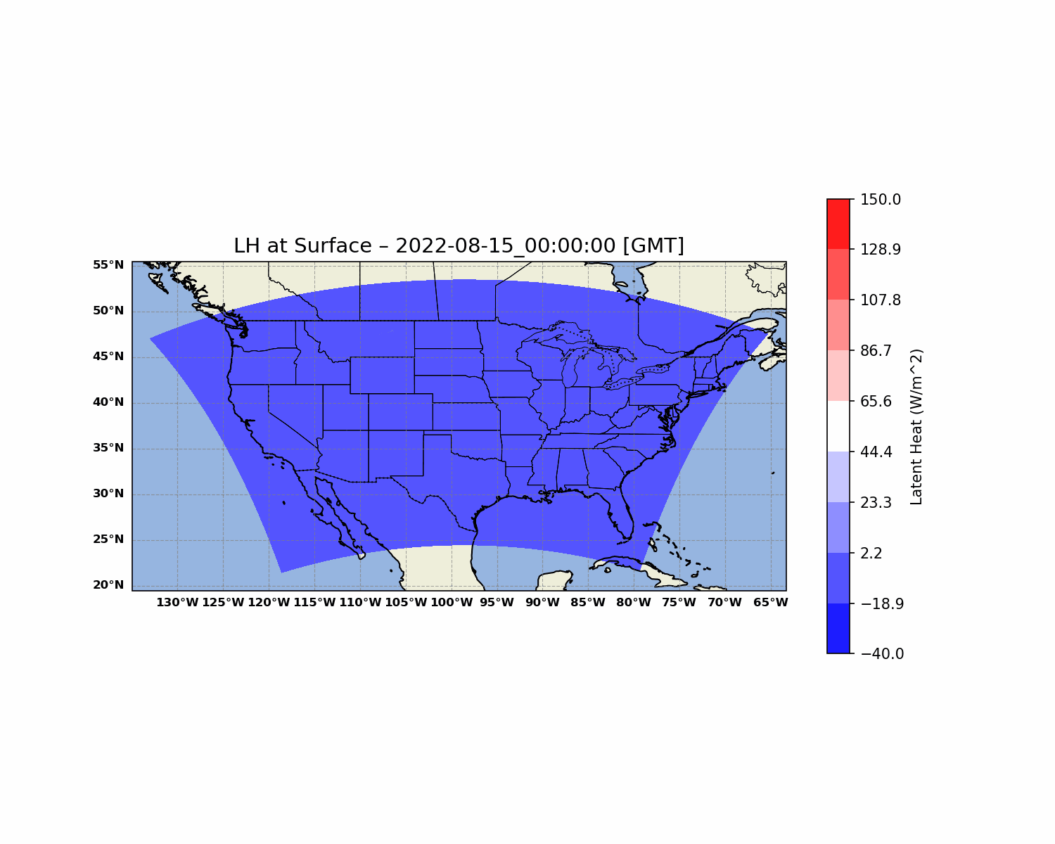
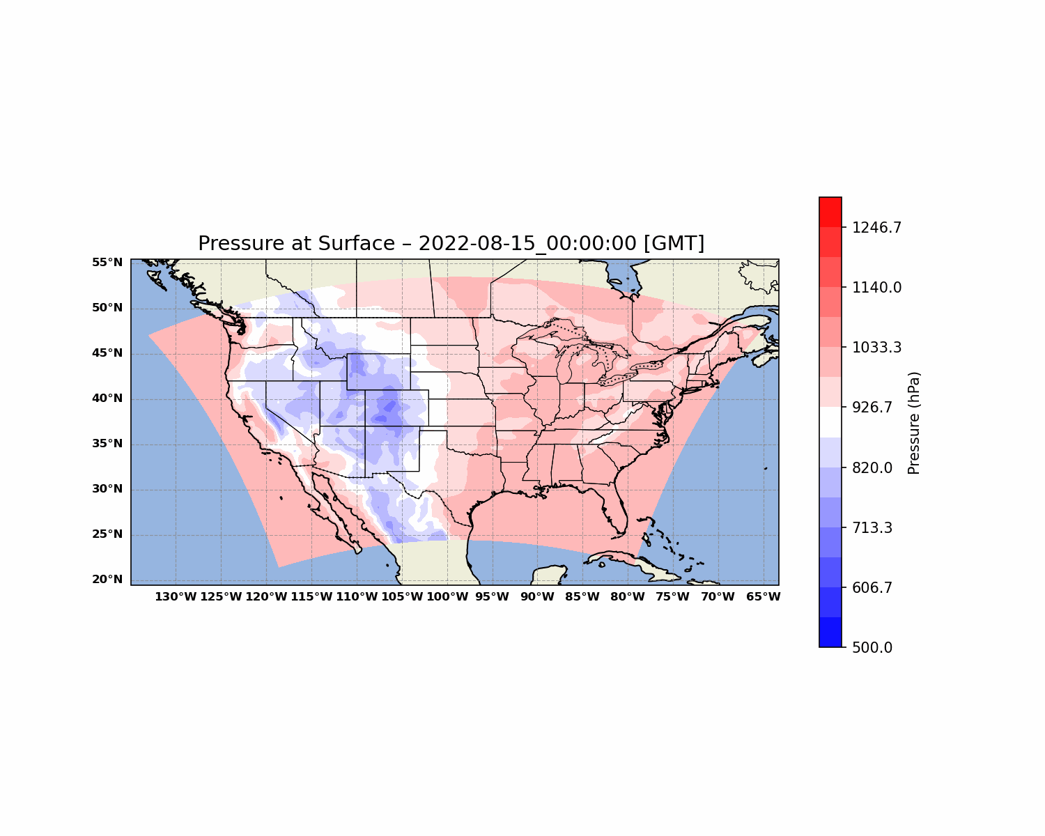
I loaded WRF output with xarray, used NumPy to derive wind-speed magnitude from U10 and V10, converted temperature and pressure units, and plotted the fields with Matplotlib and Cartopy. I compared final accumulated precipitation from RAINC + RAINNC and created sequences showing wind and latent heat flux.
Nested-domain wind-speed magnitude at three-hour intervals from August 25, 00 UTC through August 26, 21 UTC. The common color scale supports comparison through time.Surface latent heat flux at three-hour intervals from August 25, 03 UTC through August 27, 00 UTC. Colors saturate beyond ±500 W/m²; the figure does not establish that flux caused a change in storm intensity.
Interpretation and scope
This is a retrospective modeling exercise. The results have not been independently validated against observations. Comparing domain maxima alone cannot establish that the finer grid is more accurate.
Modeling, analysis, and figures: Aseem Sharma. Original coursework materials preserved from Numerical Modeling in Atmospheric Sciences.
04 / Dynamic Meteorology · Spring 2025
Visualizing atmospheric fields and evaluating WRF output
I completed the analysis and plotting for this project, using animated contour maps, domain averages, city time series, model–observation comparisons, and a wind rose to examine how atmospheric conditions vary across space and time.
Animated contour maps
Time series
Model–observation comparisons
Wind rose
WRF output
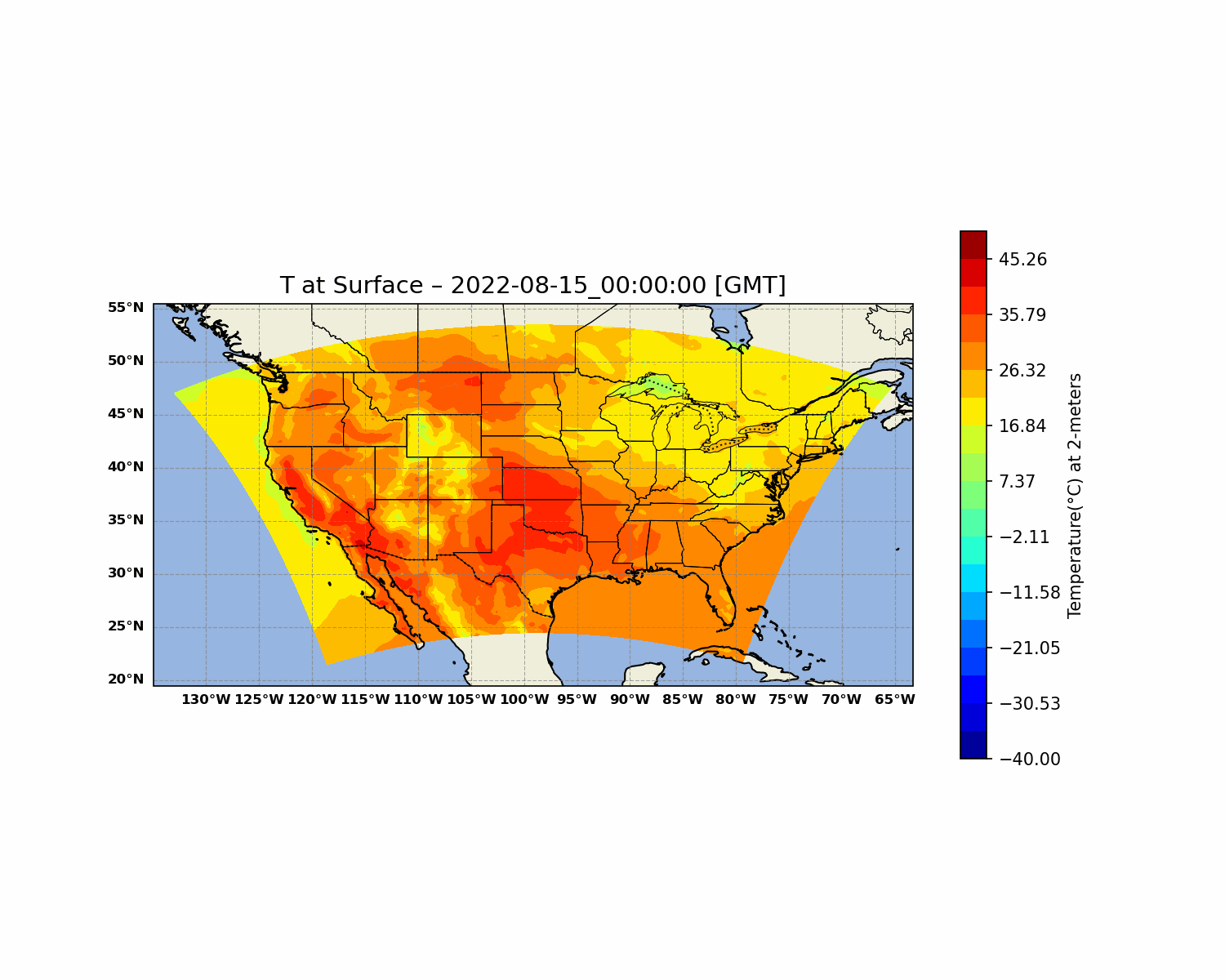
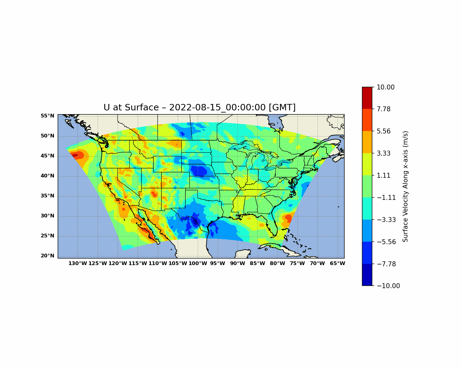
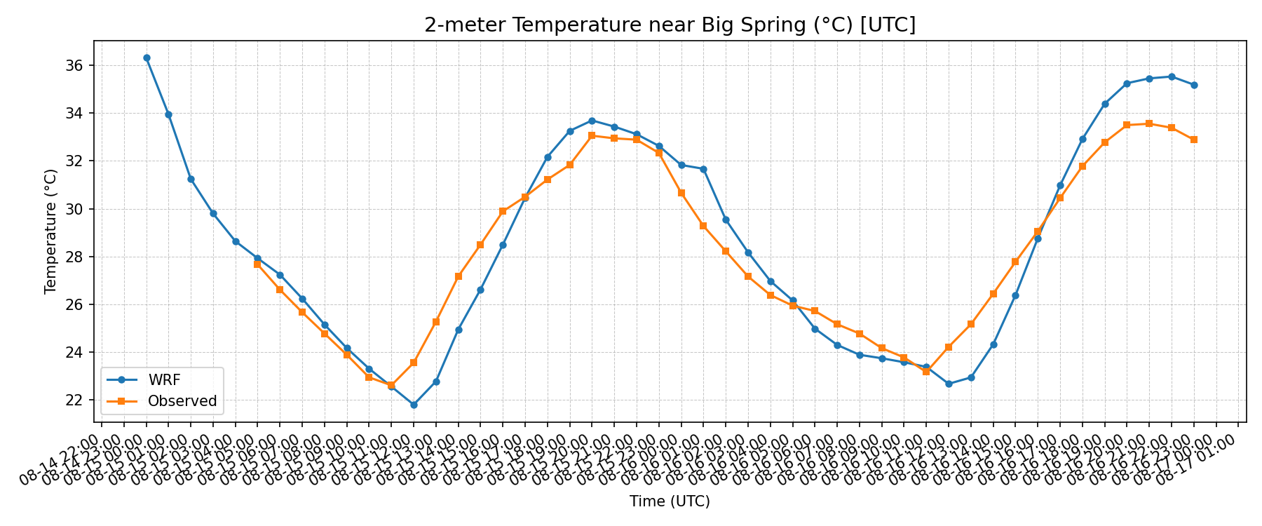
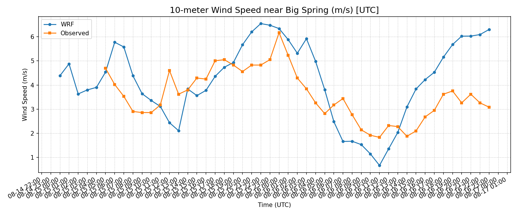
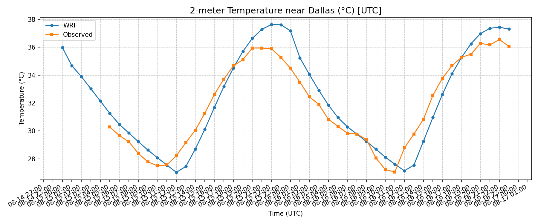
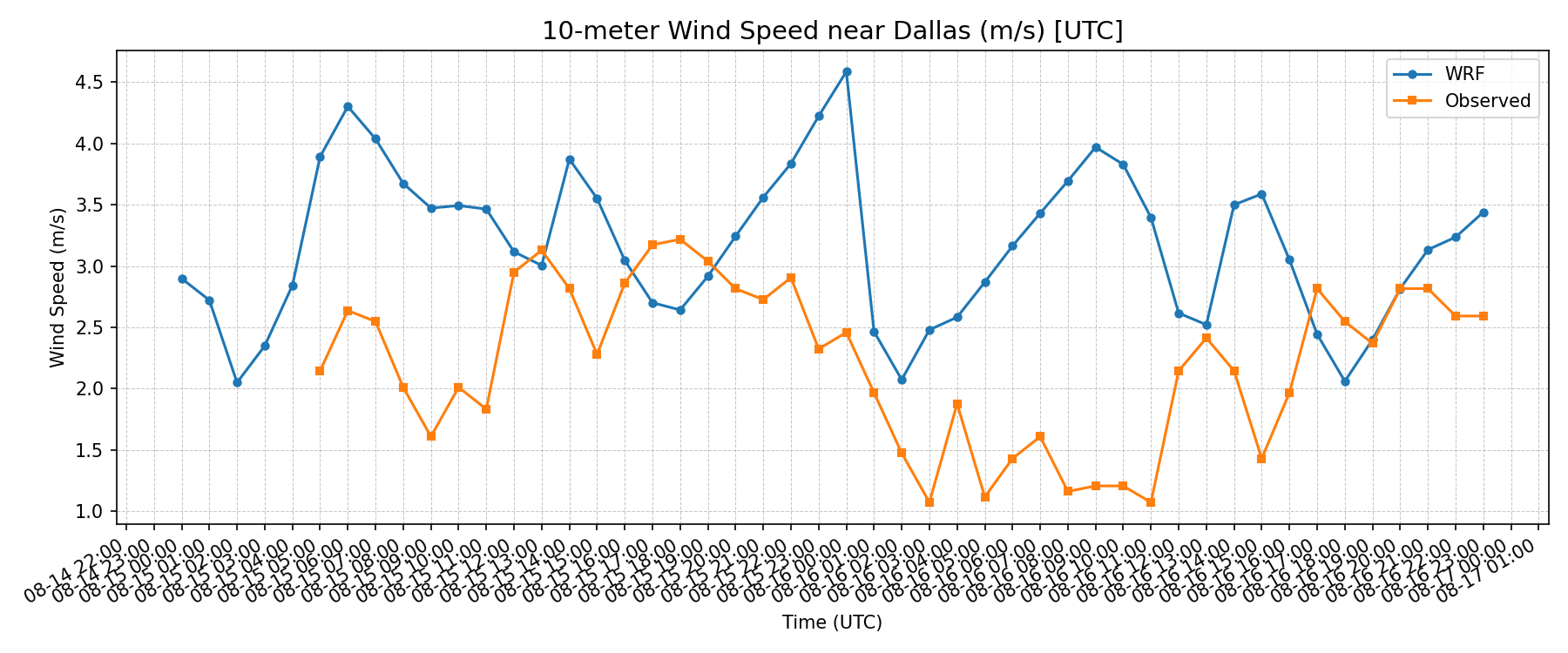
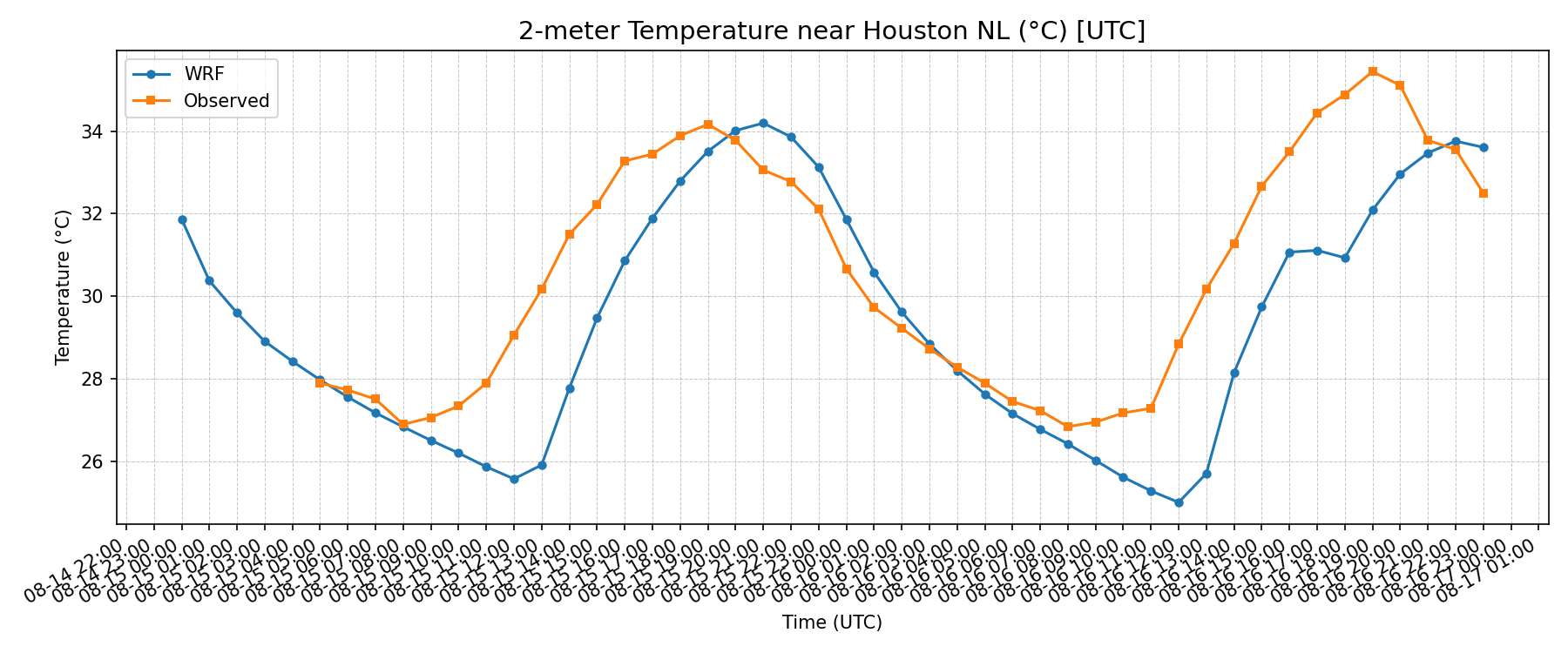
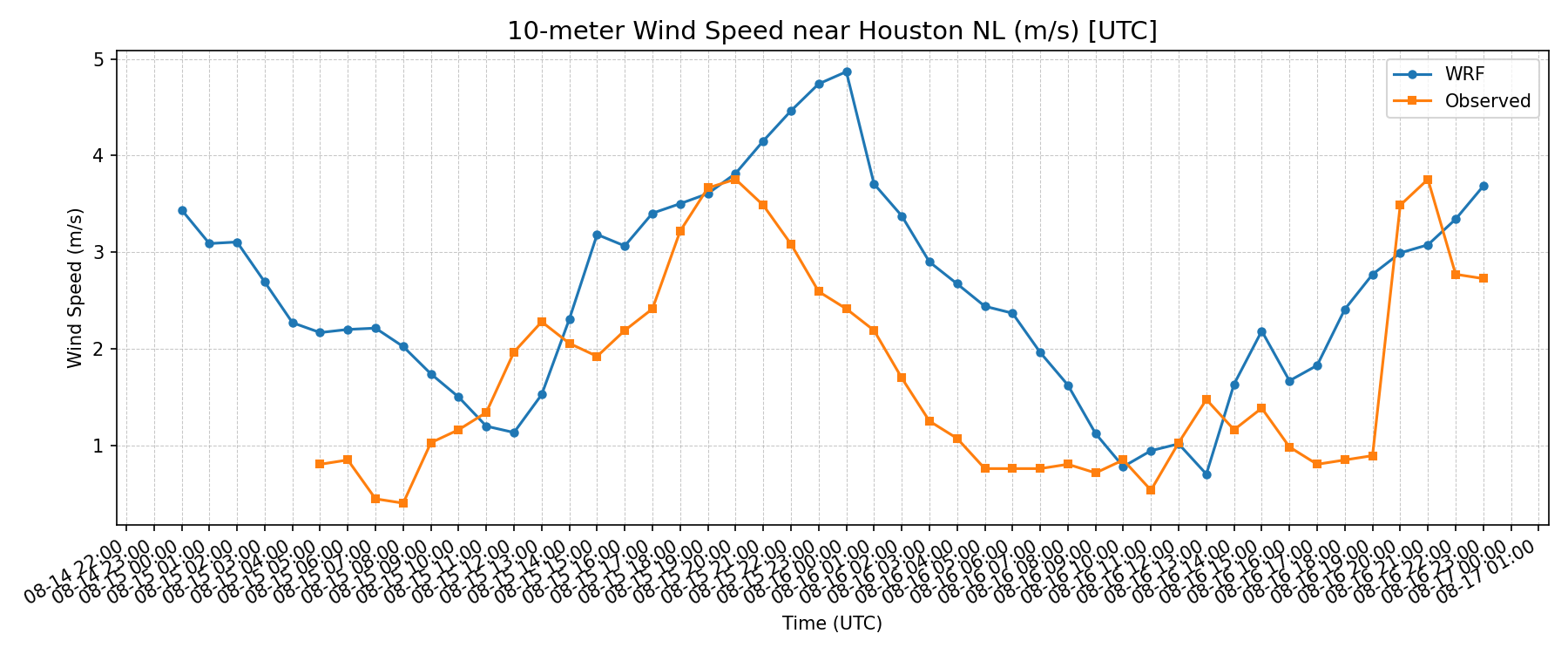
The temperature comparisons generally follow the observed daily cycle more closely than the wind-speed comparisons. The plots below show both that evaluation and the range of visualization methods used in the project.
Animated atmospheric fields
Seven map sequences show the evolution of different atmospheric variables. Play each animation individually, or open it at full resolution to inspect its axes and timestamps.
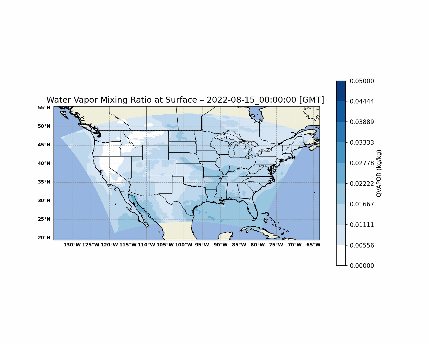
Water-vapor mixing ratio: original 49-frame sequence from the class presentation. Use the map timestamp and color scale when comparing frames.
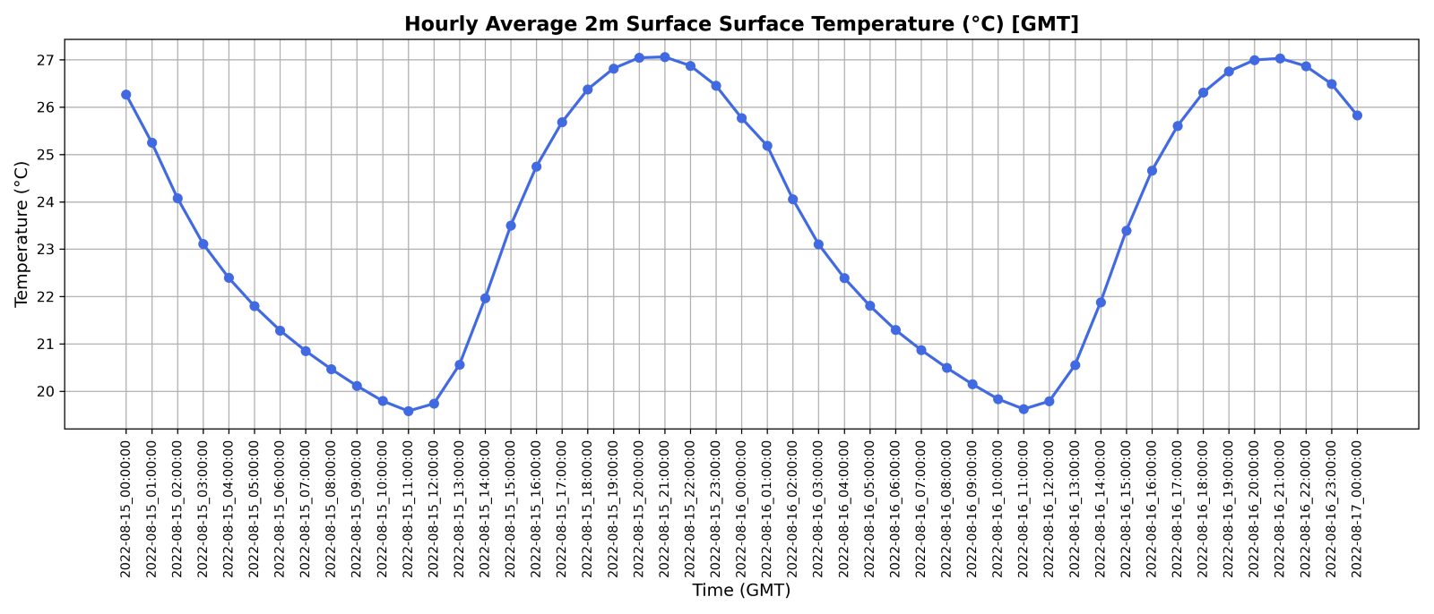
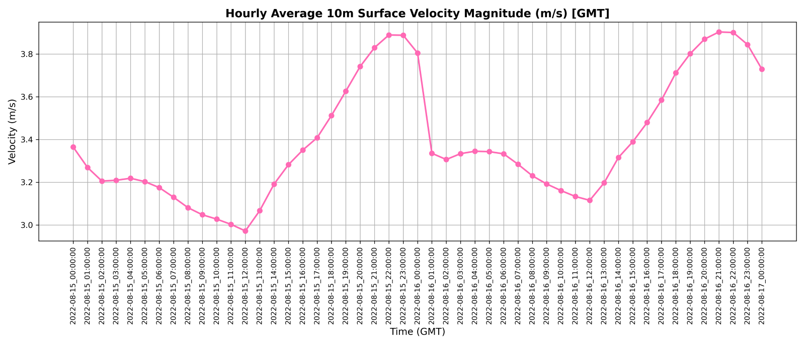
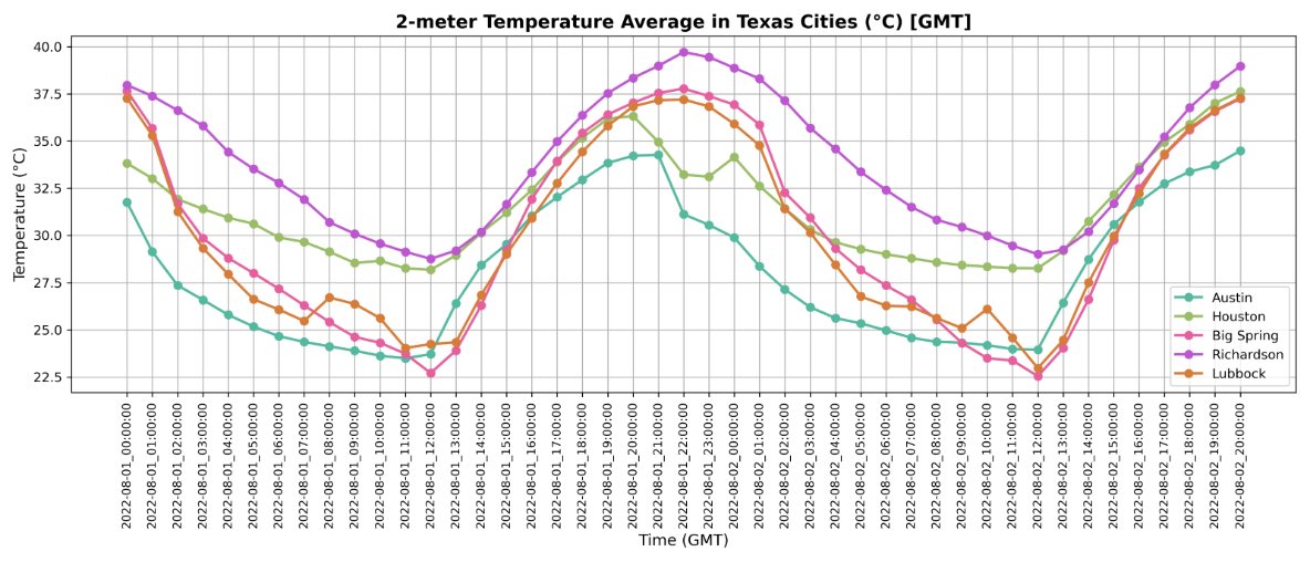
Domain averages and five-city temperature comparison · 3 plotsDomain-average two-meter temperature over the plotted interval.Domain-average ten-meter wind-speed magnitude over the plotted interval.Two-meter temperature in Austin, Houston, Big Spring, Richardson, and Lubbock; labeled August 1–2, 2022 GMT.WRF compared with observations · 6 plots
Each location has separate temperature and wind-speed comparisons. Open a figure at full size to examine its timing and units.
Big Spring
Big Spring two-meter temperature: WRF and observations.Big Spring ten-meter wind-speed magnitude: WRF and observations.
Dallas
Dallas two-meter temperature: WRF and observations.Dallas ten-meter wind-speed magnitude: WRF and observations.
Houston
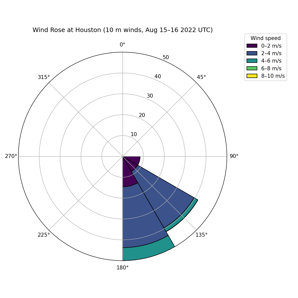
Houston two-meter temperature: WRF and observations.Houston ten-meter wind-speed magnitude: WRF and observations.Houston wind rose · Direction and speed distributionHouston wind rose, labeled August 15–16, 2022 UTC. Sectors show directional frequency and colors distinguish wind-speed categories.Study scope and credits
These are qualitative comparisons over short study periods. The city temperature chart and wind rose carry different dates and represent separate outputs. No numerical forecast-skill score is claimed. The original figures retain their labels and color scales.
Analysis and visualizations: Aseem Sharma. Figures from the original course presentation, Wonders of the Atmosphere.
05 / Environmental Data Analysis · Group project · Fall 2025
Comparing air-quality patterns in Houston and Denver
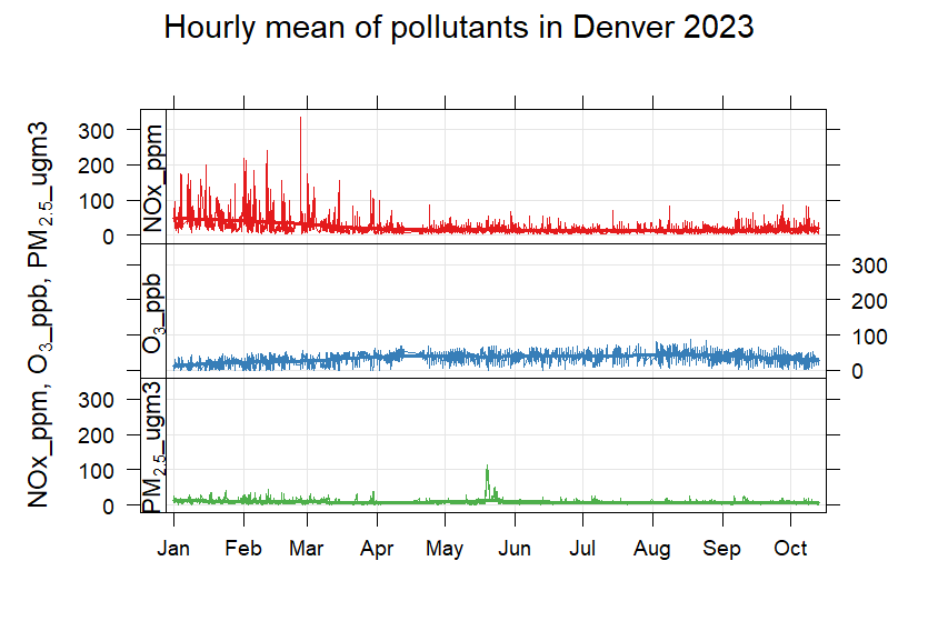
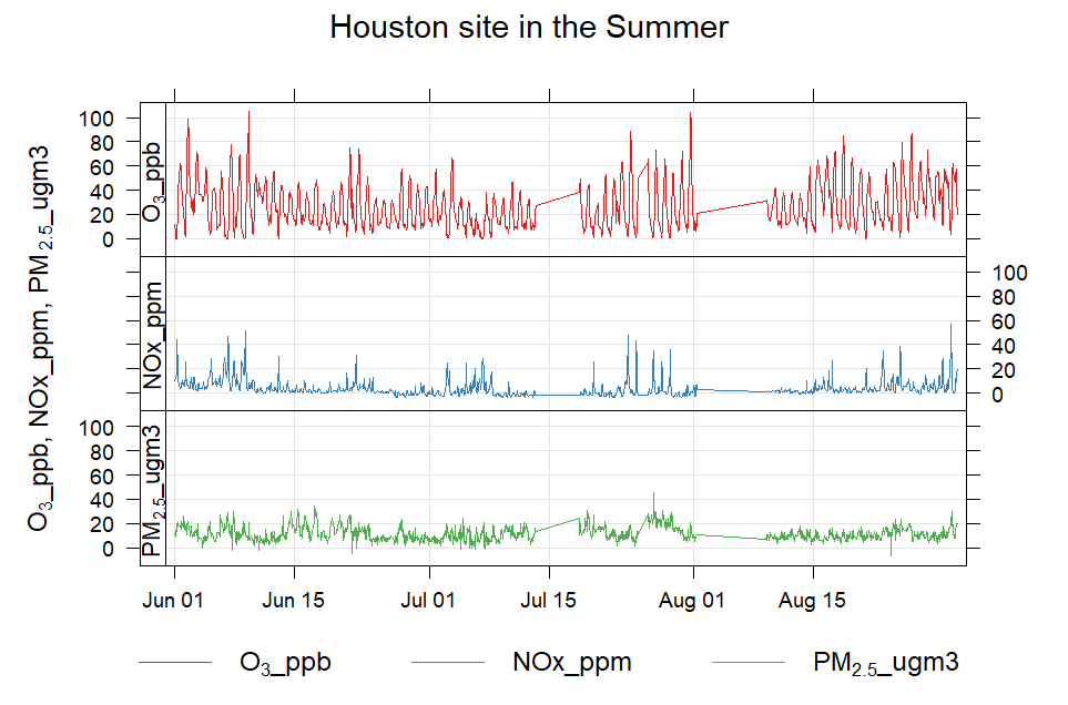
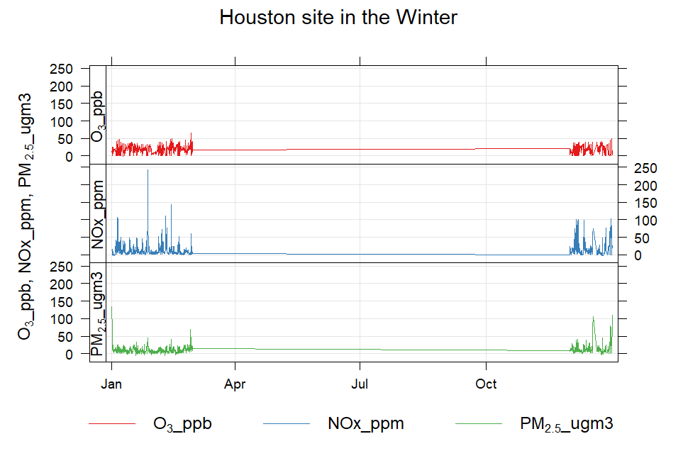
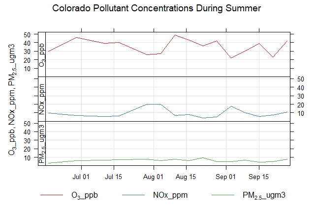
I wrote the R code and completed the analysis and plotting for this team project, using 2023 EPA AQS monitoring data to explore how pollutant concentrations vary over time at two monitoring sites. My teammates prepared the written presentation slides.
R
EPA AQS
Data preparation
Time series
Grouped comparisons
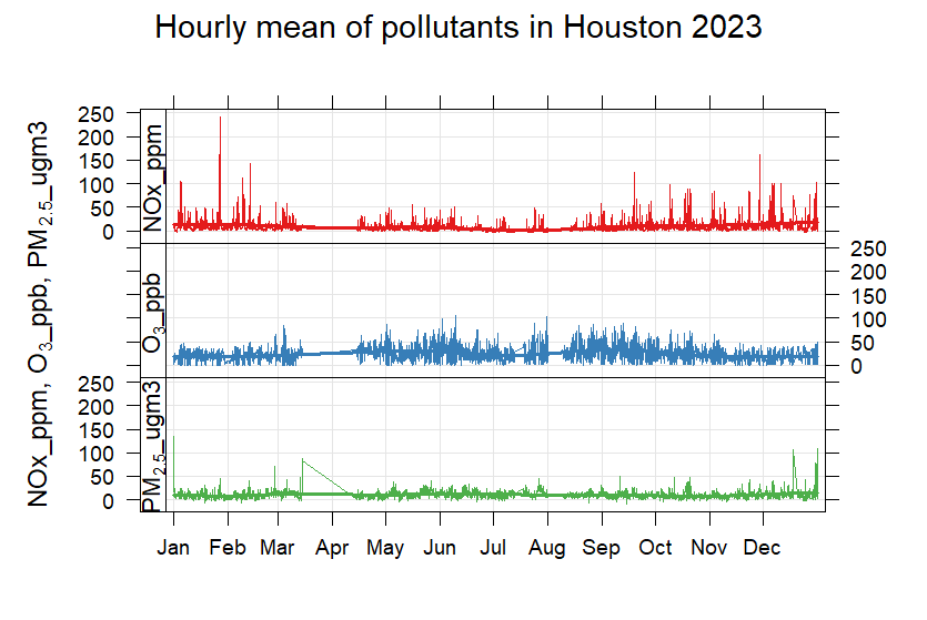
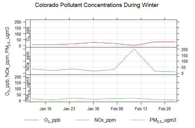
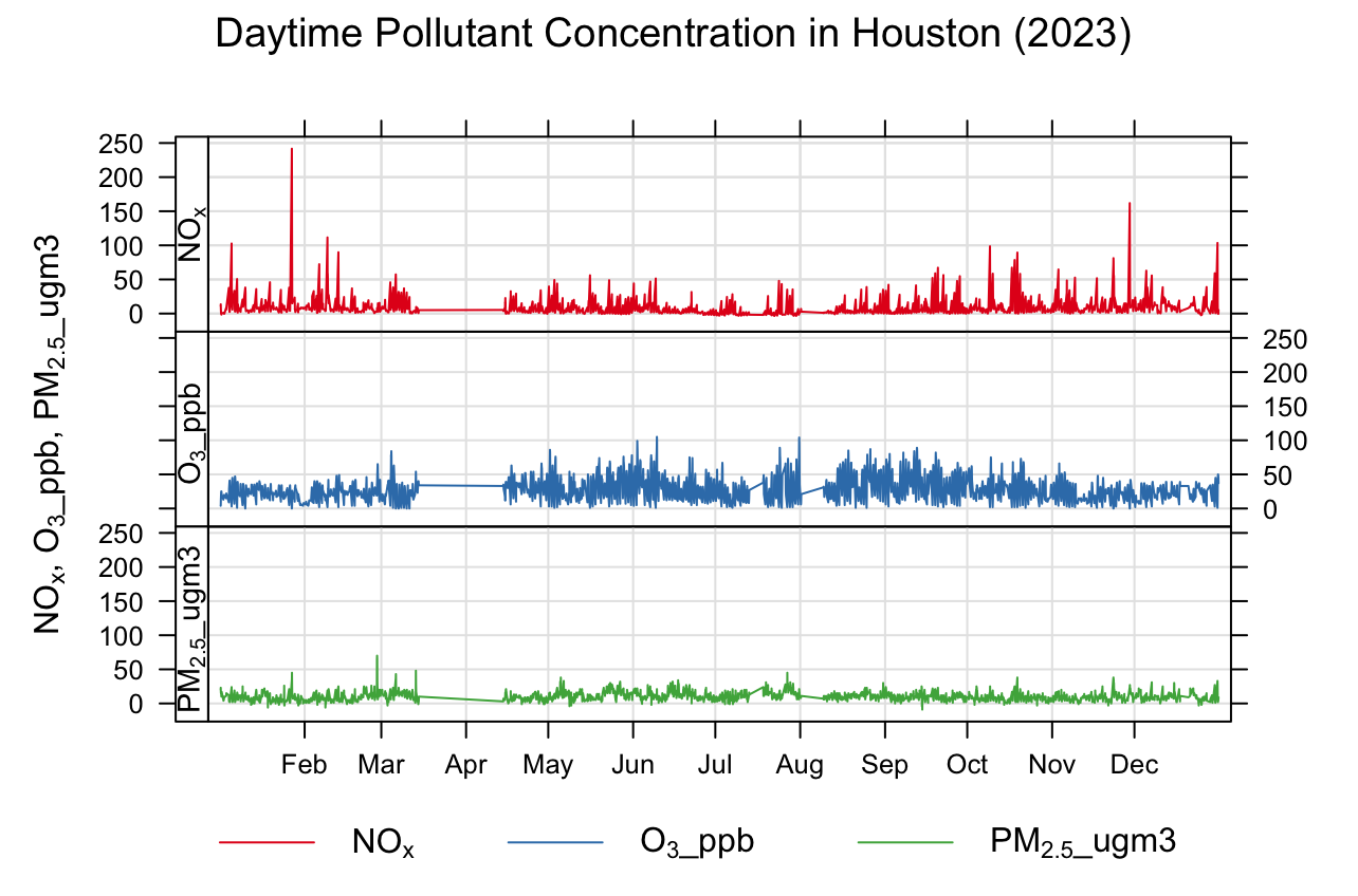
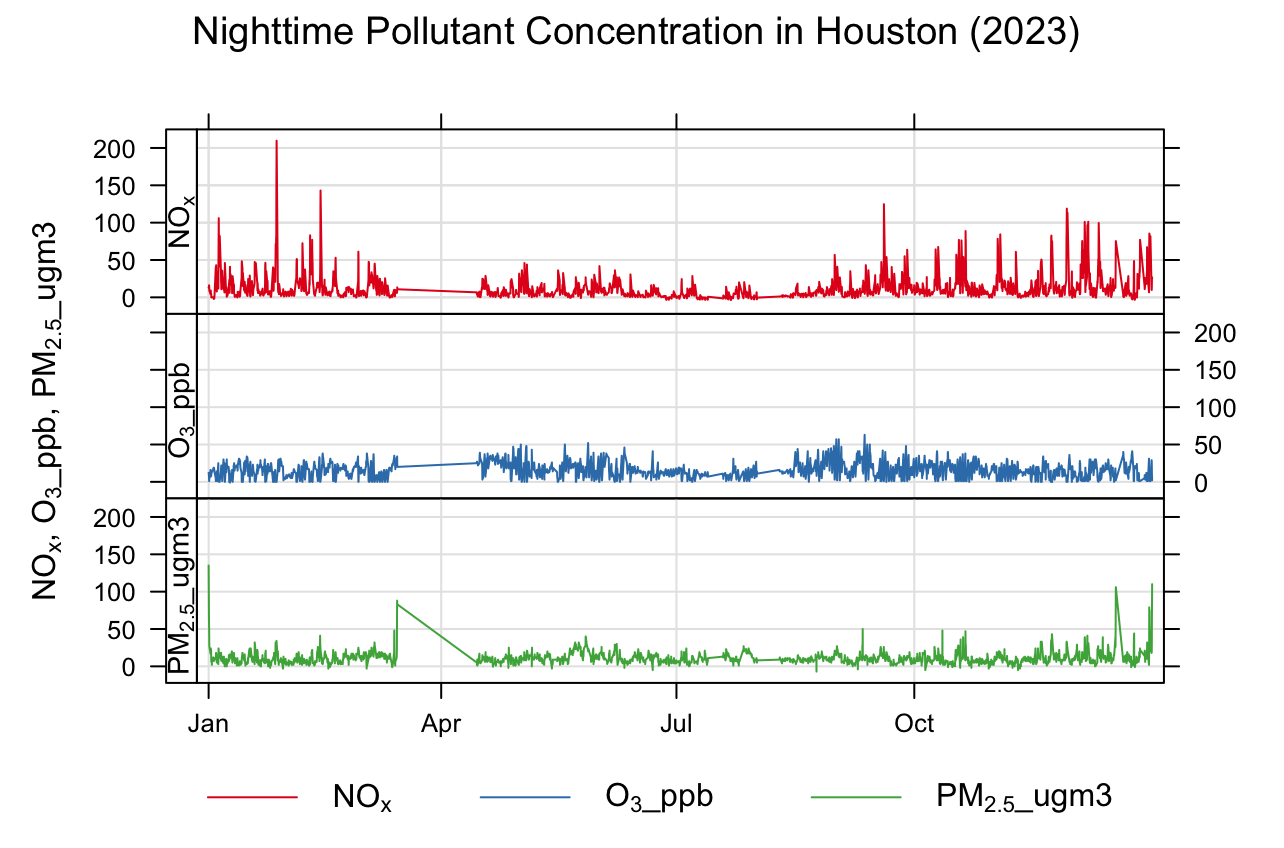
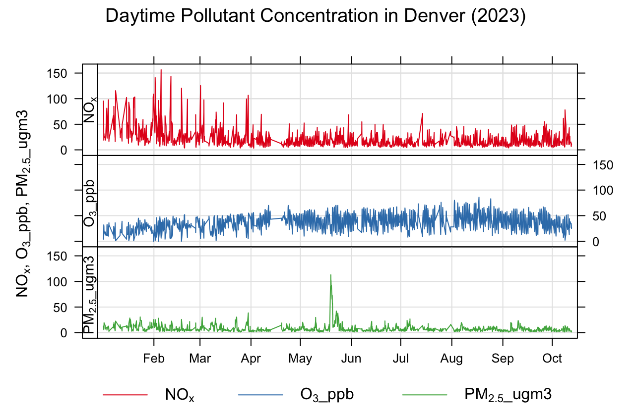
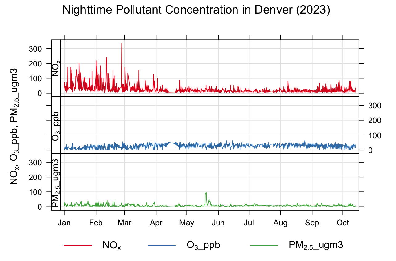
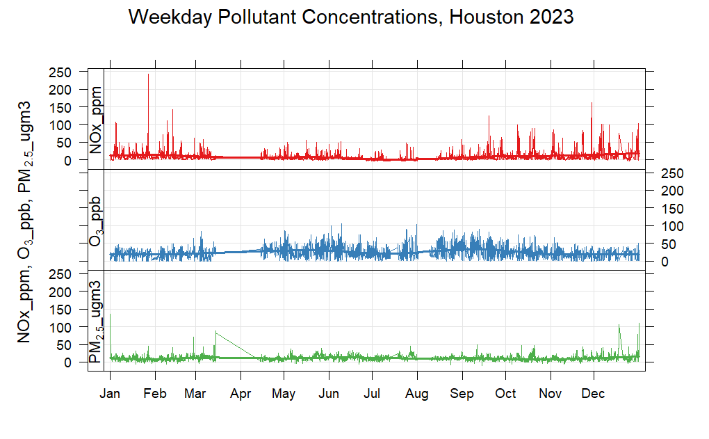
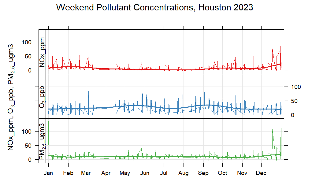
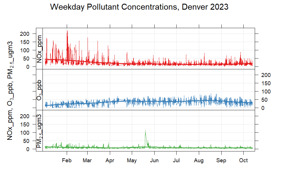
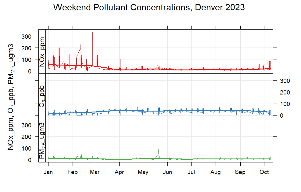
The figure collection shows several ways I organized the same environmental dataset: full-year traces, seasonal subsets, day and night, and weekdays and weekends. Select any plot to inspect the original image.
These original course figures retain their source labels. The supplied R script requests NO₂, while several plots label that series NOx. Pollutant units and the Colorado station metadata need reconciliation before interpreting numerical comparisons.
Full-year time series
Houston. Original R figure from the course presentation.Denver. Original R figure from the course presentation.
Summer and winter
Summer and winter
Houston — summer. Original R figure from the course presentation. Lines spanning gaps do not establish continuous observations.Houston — winter. Original R figure from the course presentation. Lines spanning gaps do not establish continuous observations.Colorado — summer. Original R figure from the course presentation. Lines spanning gaps do not establish continuous observations.Colorado — winter. Original R figure from the course presentation. Lines spanning gaps do not establish continuous observations.
Daytime and nighttime
Daytime and nighttime
Houston — daytime. Original R figure from the course presentation.Houston — nighttime. Original R figure from the course presentation.Denver — daytime. Original R figure from the course presentation.Denver — nighttime. Original R figure from the course presentation.
Weekdays and weekends
Weekdays and weekends
Houston — weekdays. Original R figure from the course presentation.Houston — weekends. Original R figure from the course presentation.Denver — weekdays. Original R figure from the course presentation.Denver — weekends. Original R figure from the course presentation.
06 / Numerical Modeling in Atmospheric Sciences · Fall 2025
Surface-pressure patterns in the Texas Hill Country flood case study
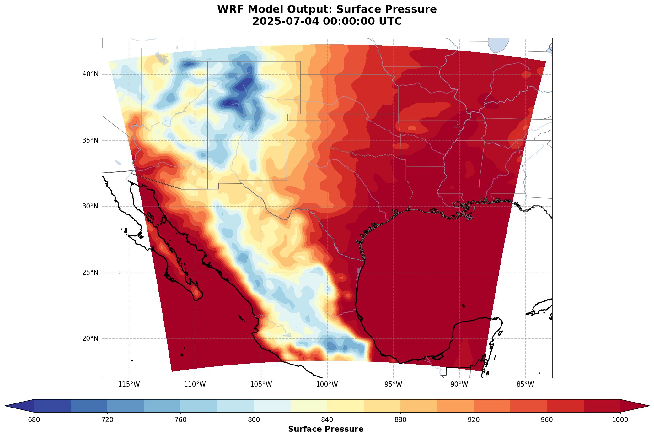
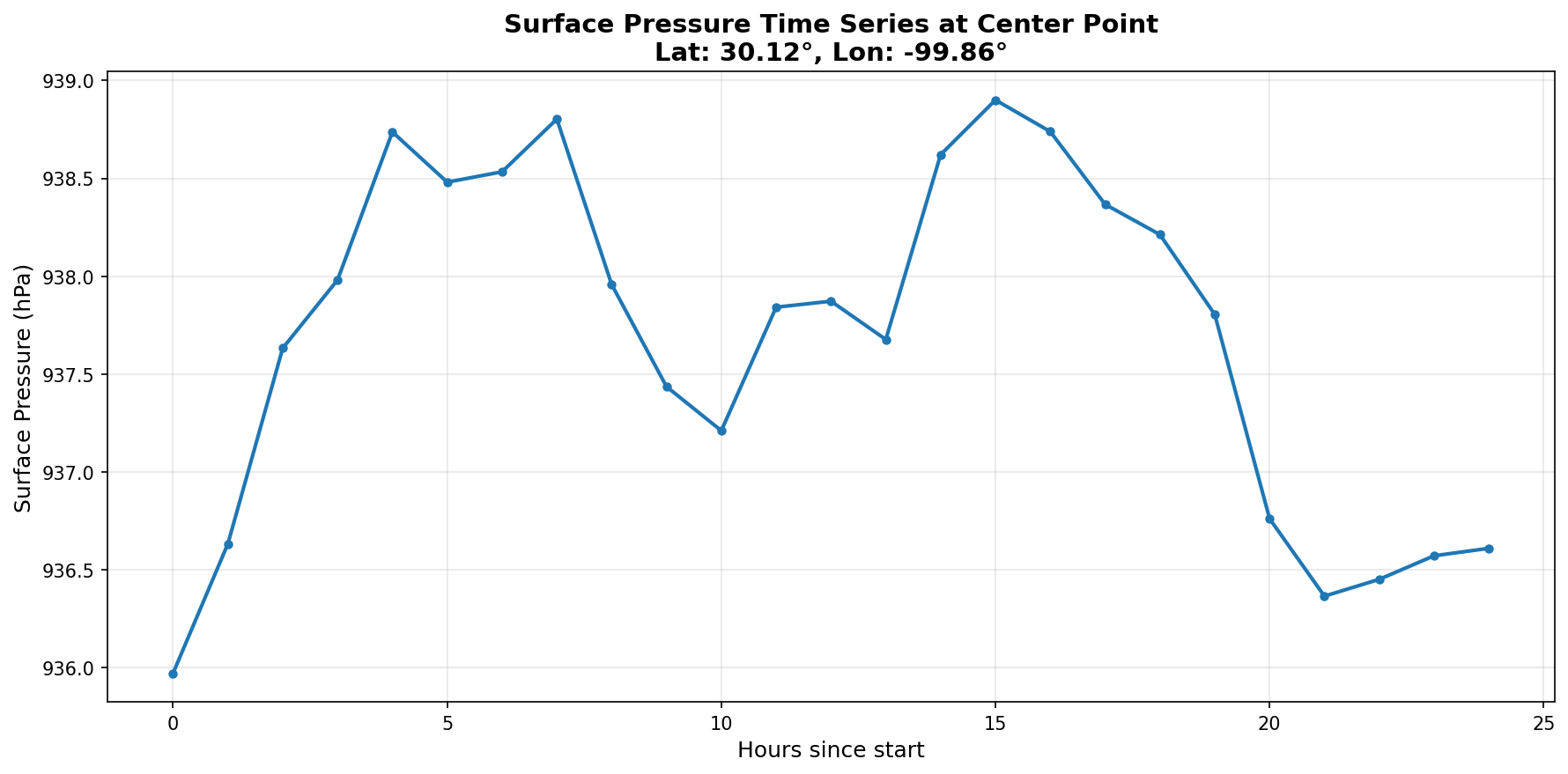
I created regional maps and a point time series from WRF output for a July 2025 Texas Hill Country flood case study. Pairing a spatial field with a local trace shows how I examined model output at different scales.
WRF output
Cartopy
Spatial visualization
Time series
Regional surface-pressure field. Original WRF map for July 4, 2025, 00 UTC. The source color bar does not specify units. Surface pressure varies with terrain elevation and is not sea-level pressure.Pressure at a selected model location. Surface pressure in hPa at 30.12° N, 99.86° W. The time axis spans hours 0–24; an absolute start time is not labeled.
Reading the two views
The map provides regional context, while the time series isolates changes at one location. These diagnostics describe atmospheric model fields; they do not measure rainfall, river flow, or flood severity.
Model-output visualization and figures: Aseem Sharma.
07 / Visual communication · UH AMS student chapter
Poster design for the UH AMS student chapter
I design the posters published on the University of Houston American Meteorological Society student chapter’s Instagram account. This work brings my interest in atmospheric science into graphic design and communication for the chapter.
A quantitative approach to environmental questions
I’m interested in roles that combine environmental science with programming and data analysis. Through my TCEQ internship and coursework, I’ve translated scientific workflows, analyzed atmospheric model output, and communicated findings through maps and time series.